이번에는 바로전에 이론적으로 확인했던 Logistic Regression에 대한 Tutorial을 진행해 보도록 하겠습니다. 지난 시간에 확인했던 내용을 잠시 요약을 해보겠습니다. Logistic Regression은 독립변수에 대해서 종속변수가 범주형의 형태를 띄는 (ex. (0, 1), (True, False)) 데이터셋에서 적용이 가능한 방법입니다.
그리고, 주요한 요소를 정리해보면... 아래와 같습니다.
Hypothesis (가설) : Sigmoid Function - 「hypothesis = P = 1 / (1 + np.exp(-f(x)))」
Loss (손실, 비용, 오차) : 「Loss = E(w) = - ∑ y * ln h(x) + (1-y) * ln (1 - h(x))」
Optimizer (최적화)
Gradient : 「Gradient = ∂E(w) = ∑ (h(x) - y) * x」
GDA : W new = W old - learning_rate * Gradient
그렇다면 데이터셋을 가정하여 생성하고, 각 방법으로 Logistic Regression을 구현해 보겠습니다.
1. Dataset 생성
2차원 좌표에 여러개의 점을찍었다고 생각하고, 어느정도 비슷한 그룹에 있는 점들에 동일한 종속변수를 부여하겠습니다. 해당 Dataset과 이를 matplotlib로 그려보면 아래와 같습니다.
import numpy as np
import matplotlib.pyplot as plt

train_x = [[1,1],[1,3],[2,2],[2,4],[3,1],[3,3],[4,2],[4,4],[5,7],[5,9],[6,6],[6,8],[7,7],[7,9],[8,6],[8,8]]
train_y = [[0],[0],[0],[0],[0],[0],[0],[0],[1],[1],[1],[1],[1],[1],[1],[1]]

train_x = np.array(train_x)
train_y = np.array(train_y)

plt.scatter(train_x[:,0:1], train_x[:,1:2], c=train_y)
plt.show()
우선 list로 생성하고, 연산을 위해서 np.array로 만들어 줍니다. 그리고 scatter plot으로 그려주는데, 이때 train_y의 그룹에 맞게 같은 그룹은 같은색으로 그려주겠습니다.

아름답게 명확하게 2개의 그룹으로 분리가 되었습니다.
2. with Numpy
Numpy를 이용한 class를 하나 생성해 줍니다. 이 안에는 3개의 메서드로 구성하고 각 메서드의 기능은 아래와 같습니다.
- fitModel( ) : train_x, train_y를 가지고 model을 학습하는 메서드
- predictModel( ) : train_x를 가지고 학습된 model의 결과에 적용해서 label을 도출하는 메서드
- evalModel( ) : test_x, test_y를 가지고 학습된 model에 적용해서 res_y를 구하고 이를 test_y와 비교한 정확도 도출
이의 전체소스는 아래와 같습니다.
class LogisticWithNumpy():
    def __init__(self):
        self.epochs = 20000
        self.learning_rate = 0.17

    def fitModel(self, x, y):
        self.w = np.random.rand(3,1) * 0.01
        eps = 1e-10

        loss_mem = []

        for e in range(self.epochs):
            logit = np.matmul(x, self.w)
            hypothesis = 1 / (1 + np.exp(-logit))
            loss = y * np.log(hypothesis + eps) + (1-y) * np.log(1 - hypothesis + eps)
            loss = -np.sum(loss)

            loss_mem.append(loss)

            gradient = np.mean((hypothesis - y) * x, axis=0, keepdims=True).T
            self.w -= self.learning_rate * gradient

        return loss_mem

    def predictModel(self, x):
        logit = np.matmul(x, self.w)
        hypothesis = 1 / (1 + np.exp(-logit))
        return hypothesis

    def evalModel(self, x, y):
        logit = np.matmul(x, self.w)
        hypothesis = 1 / (1 + np.exp(-logit))

        res_y = np.round(hypothesis, 0)
        accuracy = np.sum(res_y==y) / len(y)

        return accuracy
[주의할 점]
numpy로 적용할 때는 계산의 편의성을 위해서, weight에 bias를 추가해서 계산합니다. 따라서 train_x에 1로 구성된 열을 하나 추가해 줍니다.
train_x = np.insert(train_x, 0, 1, axis=1)[학습에 따른 loss 값 확인]
model = LogisticWithNumpy()
loss_mem = model.fitModel(train_x, train_y)

epochs_x = list(range(len(loss_mem)))
plt.plot(epochs_x, loss_mem)
plt.show()
epochs 20,000번에 learning_rate 0.17로 했을경우, loss가 더이상 줄지않고 학습이 완료 되었다고 판단이 가능합니다.
[train_x를 model에 적용하여 결과 확인]
res_y = model.predictModel(train_x)
plt.scatter(train_x[:,1:2], train_x[:,2:3], c=res_y)
plt.show()
초기에 dataset에서 확인한 내용하고 동일합니다. 결과적으로 정상적으로 도출이 됬다는것을 확인할 수 있습니다.
[정확도 결과]
test_x = [[2,3],[3,2],[6,9],[7,8],[8,7]]
test_y = [[0],[0],[1],[1],[1]]

test_x = np.insert(test_x, 0, 1, axis=1)

accuracy = model.evalModel(test_x, test_y)
print(accuracy)

#########################################
1.0
accuracy가 1.0으로 완벽하게 학습이되어, test데이터에 대해서도 정확하게 판단했습니다.
3. with Tensorflow 2.0
Tensorflow 를 이용한 class를 하나 생성해 줍니다. 이 안에는 4개의 메서드로 구성하고 각 메서드의 기능은 아래와 같습니다.
- train_on_batch( ) : batch단위로 학습할 메인 모델을 정의
- fitModel( ) : train_x, train_y를 가지고 model을 학습하는 메서드
- predictModel( ) : train_x를 가지고 학습된 model의 결과에 적용해서 label을 도출하는 메서드
- evalModel( ) : test_x, test_y를 가지고 학습된 model에 적용해서 res_y를 구하고 이를 test_y와 비교한 정확도 도출
이의 전체 소스는 아래와 같습니다.
import tensorflow as tf

print(tf.__version__)

class LogisticWithTF():
    def __init__(self):
        self.epochs = 1000
        self.learning_rate = 0.17
        self.w = tf.Variable(tf.random.normal(shape=[2,1], dtype=tf.float32))
        self.b = tf.Variable(tf.random.normal(shape=[1], dtype=tf.float32))

    def train_on_batch(self, x, y):
        with tf.GradientTape() as tape:
            logit = tf.matmul(x, self.w) + self.b
            hypothesis = tf.sigmoid(logit)
            eps = 1e-10
            loss = -tf.reduce_mean(y*tf.math.log(hypothesis+eps) + (1-y)*tf.math.log(1-hypothesis+eps))

        loss_dw, loss_db = tape.gradient(loss, [self.w, self.b])
        self.w.assign_sub(self.learning_rate * loss_dw)
        self.b.assign_sub(self.learning_rate * loss_db)

        return loss

    def fitModel(self, x, y):
        dataset = tf.data.Dataset.from_tensor_slices((x, y))
        dataset = dataset.shuffle(buffer_size=16).batch(8)

        loss_mem = []

        for e in range(self.epochs):
            for step, (x,y) in enumerate(dataset):
                loss = self.train_on_batch(x,y)
            loss_mem.append(loss)
        return loss_mem

    def predictModel(self, x):
        logit = tf.matmul(x, self.w) + self.b
        hypothesis = tf.sigmoid(logit)
        return hypothesis

    def evalModel(self, x, y):
        logit = tf.matmul(x, self.w) + self.b
        hypothesis = tf.sigmoid(logit)

        res_y = np.round(hypothesis, 0)
        accuracy = np.sum(res_y == y) / len(y)
        return accuracy
여기서 다른점은... numpy에서는 sigmoid를 수식으로 구현했으나... tensorflow는 tf.sigmoid( )로 제공하기 때문에 이를 그냥 가져다 사용합니다.
[학습에 따른 loss 값 확인]
model = LogisticWithTF()
loss_mem = model.fitModel(train_x, train_y)

epochs_x = list(range(len(loss_mem)))
plt.plot(epochs_x, loss_mem)
plt.show()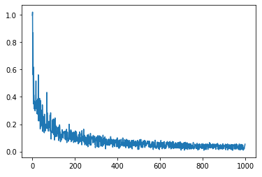
loss값이 왔다갔다 하는 모습을 보이지만 결국 최소의 값으로 수렴하고 있습니다.
[train_x를 model에 적용하여 결과 확인]
res_y = model.predictModel(train_x)
plt.scatter(train_x[:,0:1], train_x[:,1:2], c=res_y)
plt.show()
[정확도 결과]
test_x = [[2,3],[3,2],[6,9],[7,8],[8,7]]
test_y = [[0],[0],[1],[1],[1]]

test_x = np.array(test_x, dtype=np.float32)
test_y = np.array(test_y, dtype=np.float32)

accuracy = model.evalModel(test_x, test_y)
print(accuracy)

###########################################
1.0
accuracy가 1.0으로 완벽하게 학습이되어, test데이터에 대해서도 정확하게 판단했습니다.
4. with Keras
Keras 를 이용한 class를 하나 생성해 줍니다. 이 안에는 4개의 메서드로 구성하고 각 메서드의 기능은 아래와 같습니다.
- buildModel( ) : Layer를 기준으로 모델을 정의
- fitModel( ) : train_x, train_y를 가지고 model을 학습하는 메서드
- predictModel( ) : train_x를 가지고 학습된 model의 결과에 적용해서 label을 도출하는 메서드
- evalModel( ) : test_x, test_y를 가지고 학습된 model에 적용해서 res_y를 구하고 이를 test_y와 비교한 정확도 도출
이의 전체 소스는 아래와 같습니다.
class LogisticWithKeras():
    def __init__(self):
        self.epochs = 500
        self.learning_rate = 0.17

    def buildModel(self):
        self.model = tf.keras.Sequential()
        self.model.add(tf.keras.layers.Dense(1, activation='sigmoid'))

        optimizer = tf.keras.optimizers.SGD(self.learning_rate)

        self.model.compile(loss='binary_crossentropy', optimizer=optimizer, metrics=['binary_accuracy'])

    def fitModel(self, x, y):
        self.model.fit(x, y, epochs=self.epochs, batch_size=8, shuffle=True)

    def predictModel(self, x):
        return self.model.predict(x)

    def evalModel(self, x, y):
        return self.model.evaluate(x,y)
[학습에 따른 loss 값 확인]
model = LogisticWithKeras()
model.buildModel()
model.fitModel(train_x, train_y)
Epoch 990/1000
16/16 [==============================] - 0s 507us/sample - loss: 0.0324 - binary_accuracy: 1.0000
Epoch 991/1000
16/16 [==============================] - 0s 493us/sample - loss: 0.0323 - binary_accuracy: 1.0000
Epoch 992/1000
16/16 [==============================] - 0s 528us/sample - loss: 0.0333 - binary_accuracy: 1.0000
Epoch 993/1000
16/16 [==============================] - 0s 494us/sample - loss: 0.0343 - binary_accuracy: 1.0000
Epoch 994/1000
16/16 [==============================] - 0s 466us/sample - loss: 0.0338 - binary_accuracy: 1.0000
Epoch 995/1000
16/16 [==============================] - 0s 443us/sample - loss: 0.0322 - binary_accuracy: 1.0000
Epoch 996/1000
16/16 [==============================] - 0s 499us/sample - loss: 0.0327 - binary_accuracy: 1.0000
Epoch 997/1000
16/16 [==============================] - 0s 503us/sample - loss: 0.0325 - binary_accuracy: 1.0000
Epoch 998/1000
16/16 [==============================] - 0s 469us/sample - loss: 0.0339 - binary_accuracy: 1.0000
Epoch 999/1000
16/16 [==============================] - 0s 465us/sample - loss: 0.0326 - binary_accuracy: 1.0000
Epoch 1000/1000
16/16 [==============================] - 0s 418us/sample - loss: 0.0348 - binary_accuracy: 1.0000loss가 매우 낮은 수준으로 안정되었고... 정확도가 1.0으로 성공적으로 학습되었습니다.
[train_x를 model에 적용하여 결과 확인]
res_y = model.predictModel(train_x)
plt.scatter(train_x[:,0:1], train_x[:,1:2], c=res_y)
plt.show()
계속 보시면 알겠지만, class만 변경되고 나머지 실행코드는 동일합니다.
[정확도 결과]
test_x = [[2,3],[3,2],[6,9],[7,8],[8,7]]
test_y = [[0],[0],[1],[1],[1]]

test_x = np.array(test_x, dtype=np.float32)
test_y = np.array(test_y, dtype=np.float32)

print(model.evalModel(test_x, test_y))

###########################################
5/5 [==============================] - 0s 12ms/sample - loss: 0.0075 - binary_accuracy: 1.0000
[0.007485953159630299, 1.0]
accuracy가 1.0으로 완벽하게 학습이되어, test데이터에 대해서도 정확하게 판단했습니다.
이렇게 3가지로 구현해 보았습니다. 앞으로는 현재 Tensorflow에서 인정한 유일한 high level api인 keras만을 사용해서 구현해 보겠습니다.
-Ayotera Lab-
댓글